
Bike Sharing Machine Learning Model
Published in MDS-UBC GitHub, 2020
Demand forecasting is an important aspect for many companies in carrying out their operations. In this project we analyze the bike-sharing dataset from UCI Machine Learning Repository, and build a regression learning machine model using the Random Forest Regressor algorithm to predict the count of bike rentals based on time and weather-related information. For this project we use Docker, making it easier to replicate the analysis.
$\bigstar$ Click here to look at the original GitHub repository of this project.
Authors: Aman Kumar (amank90), Dora Qian (doraqmon), and Victor Cuspinera (vcuspinera)
Dataset
The data that we use to build the model comes from the bike-sharing dataset created by Dr. Hadi from LIAAD and shared in the UCI Machine Learning Repository.
This dataset contains the hourly information about the numbers of bike rentals in Washington, DC between 2011 and 2012. It has 17 variables, standing out:
cnt(our target) count of total rental bikes including both casual and registeredseason: Season (1:spring, 2:summer, 3:fall, 4:winter)dteday: Datehr: Hourholiday: (0: No, 1: Yes)weekday: Day of the week (starting from 0: Sunday)workingday: (0: No, 1: Yes)weathersit: (1: Sunny or partly cloudy. 2: Mist or cloudy. 3: Light rain or snow. 4: Heavy rain, thunderstorm or snow)temp: Normalized temperature in Celsiushum: Normalized humiditywindspeed: Normalized wind speed
Explanatory Data Analysis (EDA)
In this initial analysis, we separate the dataset in two parts: train and test. Afterwards, we built some visualizations to deep dive the data and found the relationships between different variables, as well as the explanatory variables with a higher correlation with the target variable (number of bikes rented). The full EDA report can be found here.
Among our finds, we observe that the demand for bikes increases when the weather is warmer and decreases when the temperatures are lower.
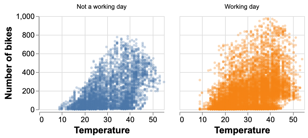
Figure 1. Analysis of temperatures by working day
The day of week and hour of the day clearly affects the count of bike rental. Also, people rent these bikes mainly for work and school on weekdays showing the peak of the demand in two times of the day. Besides, people use rental bikes between 11 am and 4 pm during weekends.
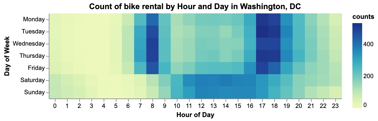
Figure 2. Analysis per hour and weekday
The correlation matrix between features, including the target variable, is shown below.
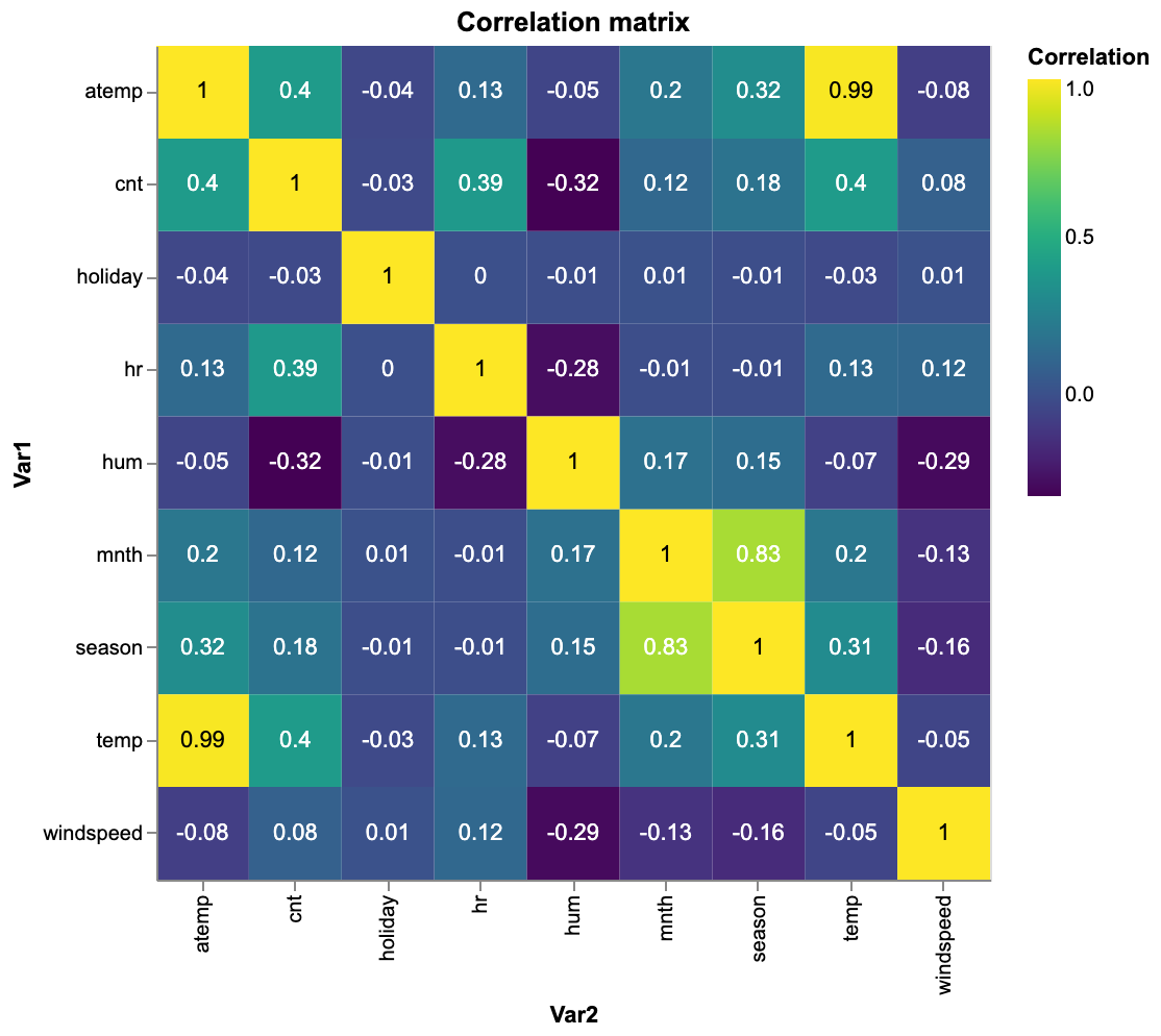
Figure 3. Correlation matrix
Analysis
The original dataset has categorical features preprocessed using label encoding and numerical features preprocessed using MinMaxScalar. So, we decide to de-normalize the numerical features before splitting the data in train and test datasets. Also, we changed holiday and workingday to OneHotEncoding.
For the analysis we test different models from Scikit-learn, tunning different hyperparameters (i.e. ‘max_depth’ and ‘n_estimators’) which were chosen used 5-fold cross-validation with mean squared error as the regression metric.
For this project we use both the R and Python programming languages, R mainly for Data Wrangling and Python for Model Selection.
Results
To choose the best prediction model, we test the Linear Model Regression, KNN and Random Forest from Scikit-learn and choose the one that returns the best score in the test dataset, comparing the mean_squared_error and the error for both training and testing error. The full final report can be found here.
| Model | Train.Error | Test.Error | Train.r2.score | Test.r2.score | Best.Parameters | Computational.Time..sec. |
|---|---|---|---|---|---|---|
| LinearRegression | 147.91 | 145.61 | 0.34 | 0.35 | {‘normalize’: False} | 0.09 |
| KNN | 72.19 | 78.43 | 0.84 | 0.81 | {‘n_neighbors’: 15} | 1.51 |
| RandomForest | 63.88 | 70.71 | 0.88 | 0.85 | {‘max_depth’: 10, ‘n_estimators’: 50} | 127.88 |
As we can see above, Random Forest is the best model with minimum training and testing error. By hyperparameter tuning, we get best hyper parameters as max_depth: 10, and n_estimators: 50.
It is possible to see the feature importance through random forest regression.
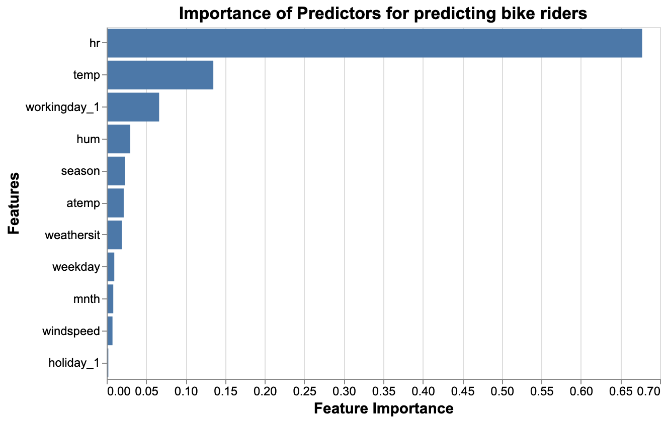
Figure 4: The plot for importance for predictors.
The variable hr is the most important feature to predict bike ridership. The second most important feature is temp.
In order to visualize the results, we also compared in the next plot the between real rides from test dataset vs. the predicted rides from our Random Forest model.
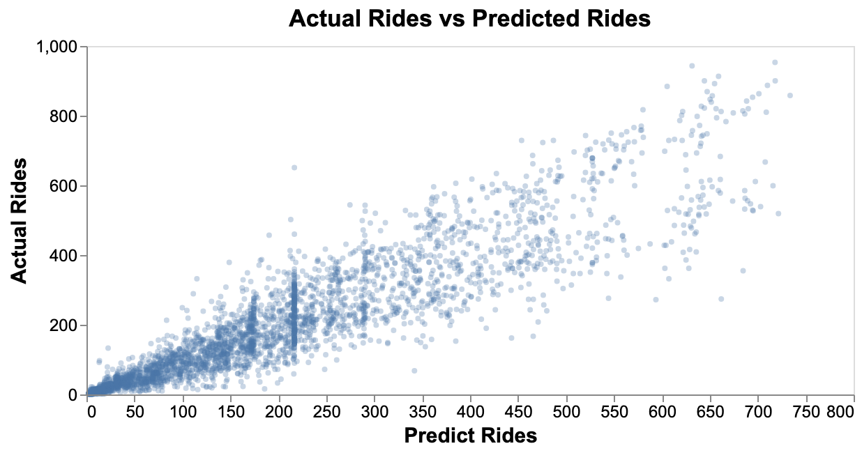
Figure 5: The plot for predicted and actual rides
The relationship looks very linear which means that the predicted values are close to the actual values. The model can be used to predict the ridership in the future given the input features.
In order to improve our model further, we can perform more feature engineering.